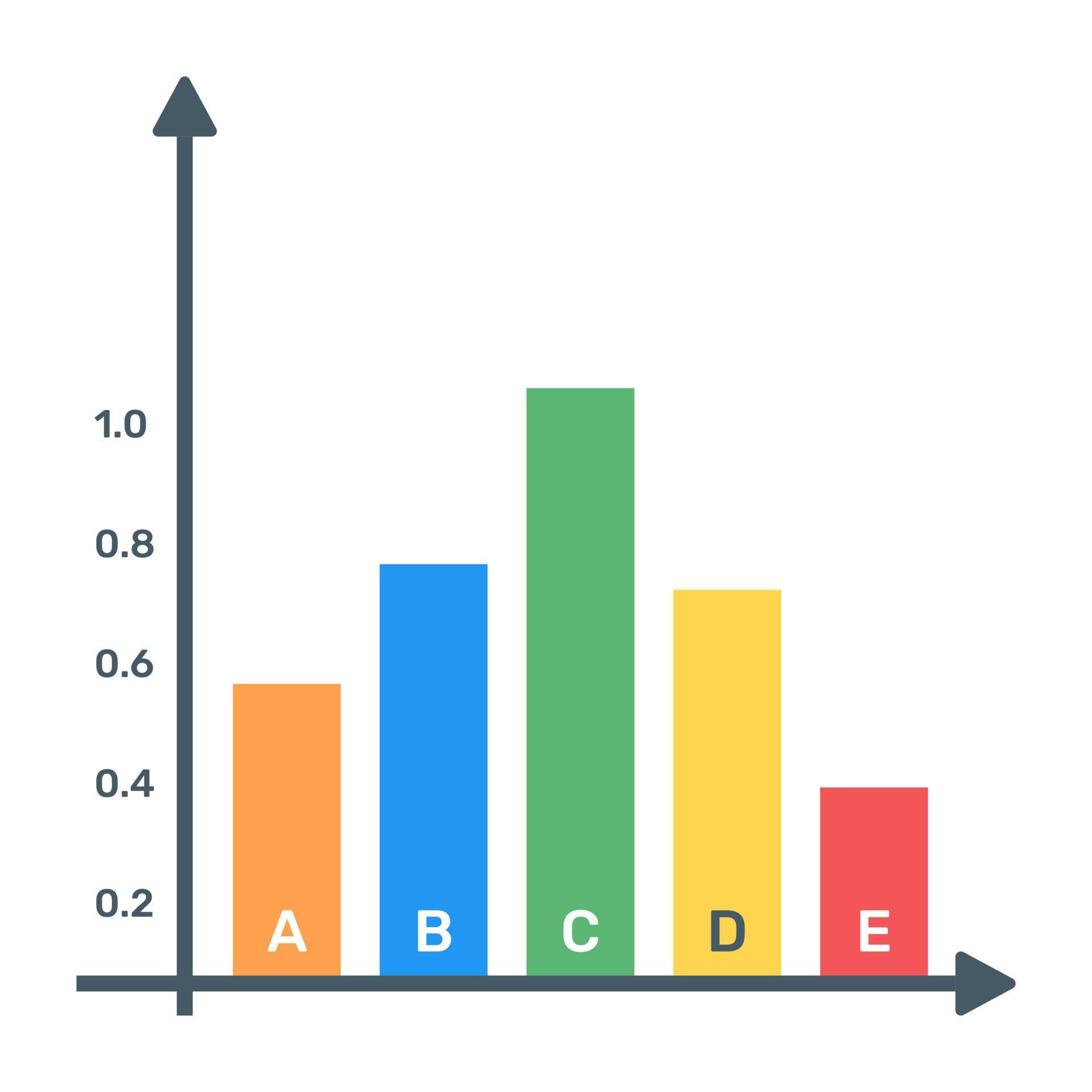
Gráfico $e/y_c$ Vs. $y/y_c$

Understanding the nuances of the gráfico $e/y_c$ vs. $y/y_c$ is essential for anyone working with dynamic economic or engineering models that compare equilibrium states to current outputs.

What Does $e/y_c$ Represent in Analytical Diagrams?

The ratio $e/y_c$ serves as a powerful normalized metric that expresses the deviation of a structural error or shock (e) relative to the capacity or steady-state level (y_c). In a gráfico $e/y_c$ vs. $y/y_c$, this term usually appears on the horizontal axis, providing a standardized measure that is independent of units. By expressing the disturbance as a proportion of the system’s potential, analysts can compare scenarios across different scales or sectors without confusion. This normalization highlights how large a shock is relative to what the system can reasonably absorb.

From a modeling perspective, $e$ often stands for an unexpected perturbation, such as a technological disruption, a policy shock, or a transient market inefficiency. The denominator $y_c$, representing capacity or a long-run equilibrium level, anchors the ratio in a meaningful baseline. When you plot $e/y_c$, you are effectively asking: “How disruptive is this shock in relation to the system’s normal operating ceiling?” This framing is common in robustness checks for macroeconomic simulations and in engineering diagnostics where residual errors are scaled by design limits.

What Does $y/y_c$ Represent in Comparative Visualizations?

On the vertical axis of the gráfico $e/y_c$ vs. $y/y_c$, the term $y/y_c$ captures the current state of the system relative to its ideal or full-capacity level. Here, $y$ denotes the observed output, while $y_c$ again acts as the benchmark, whether that is a physical capacity, a natural level of output, or a theoretical equilibrium. This ratio is particularly useful because it immediately signals whether the system is underperforming, performing at target, or exceeding expectations.

When analysts study the trajectory of $y/y_c$, they gain insight into dynamics such as utilization rates, efficiency gaps, or cyclical positions. For instance, a value below one indicates a shortfall, whereas a value above one may suggest overheating or unsustainable strain. In the combined gráfico $e/y_c$ vs. $y/y_c$, this axis allows researchers to see how deviations from normal performance align with the size of disturbances, creating a clear visual language for diagnosis and forecasting.

Why Compare These Two Ratios in One Graph?

Placing $e/y_c$ and $y/y_c$ on the same axes transforms abstract equations into a diagnostic tool that is both intuitive and informative. The gráfico $e/y_c$ vs. $y/y_c$ essentially maps shock intensity against current utilization, revealing whether observed outcomes are driven by temporary disturbances or by structural shifts. This dual-axis perspective is invaluable for policymakers, engineers, and analysts who need to distinguish between noise and signals in complex systems.

Such comparisons also support clearer communication across teams. A single visual can convey whether a factory is running below capacity due to a minor glitch or a major breakdown, or whether an economy is experiencing a mild slowdown versus a deep recession. By reducing multidimensional data to two interpretable ratios, the graph becomes a versatile instrument for scenario analysis, stress testing, and strategic planning.

Interpreting the Shape and Clusters in the Graph

In a well-constructed gráfico $e/y_c$ vs. $y/y_c$, patterns quickly emerge that guide decision-making. Points clustered near the origin suggest small disturbances and output close to potential, indicating a stable regime. Conversely, points in the upper-right quadrant reveal high disturbance levels alongside strong performance, which might signal an unsustainable boom or an inefficient push beyond normal limits.

Downward-sloping clusters can imply that larger shocks are associated with underperformance, highlighting vulnerabilities in the system. Outliers in the upper-left quadrant, where disturbance is low but output is high, may denote exceptional efficiency or data anomalies worth investigating. By regularly updating this graph, organizations can monitor shifts in these clusters over time, adapting strategies as the underlying dynamics evolve.

Practical Applications Across Disciplines

The versatility of the gráfico $e/y_c$ vs. $y/y_c$ makes it applicable in numerous fields, from economics and finance to operations and environmental science. Central banks might use it to assess the impact of policy shocks on actual GDP relative to potential output. Engineers could apply it to monitor machine performance, comparing unexpected errors to design tolerances. Supply chain managers may rely on it to visualize disruptions against throughput capacity, enabling more resilient planning.

Academics also benefit from this framework when presenting theoretical models, as it simplifies complex relationships into an accessible visual format. Students and practitioners alike can explore how changes in $e$ and $y$ propagate through the system, fostering a deeper intuition for stability, resilience, and optimal operation. The graph thus becomes not only an analytical device but also a teaching tool that bridges theory and practice.

Best Practices for Building and Using This Graph

To get the most out of a gráfico $e/y_c$ vs. $y/y_c$, it is important to define $y_c$ clearly and consistently, whether it is based on historical averages, engineering specifications, or equilibrium theory. The numerator $e$ should be carefully constructed, often as a residual or de-trended component, to ensure that the ratio reflects meaningful deviation rather than measurement noise. Proper scaling, labeling, and color coding further enhance readability, especially when comparing multiple sectors or time periods.

Interactive versions of the graph, where users can hover over points to see dates or contextual events, can dramatically improve its utility. Regular updates, combined with clear documentation of assumptions, help maintain credibility and relevance. When used thoughtfully, this visual tool supports smarter decisions, highlights hidden risks, and invites richer conversations about how a system performs under varying conditions.

In summary, the gráfico $e/y_c$ vs. $y/y_c$ is more than a technical diagram; it is a concise narrative of how disturbances interact with capacity, turning complex data into actionable insight across economics, engineering, and management.